Navigating with Semantic Segmentation

• Overview

• Requirements

• Semantic Segmentation Overview

• Tutorial Steps

• Conclusion

Overview

This tutorial demonstrates how to use semantic segmentation in costmaps with stereo cameras, using a custom semantic_segmentation_layer plugin and a pre-trained segmentation model that works on Gazebo’s Baylands world. It was written by Pedro Gonzalez at robot.com.

Requirements

It is assumed ROS2 and Nav2 dependent packages are installed or built locally. Additionally, you will need:

source /opt/ros/<ros2-distro>/setup.bash
sudo apt install ros-$ROS_DISTRO-nav2-minimal-tb4*
sudo apt install ros-$ROS_DISTRO-ros-gz-sim
sudo apt install ros-$ROS_DISTRO-ros-gz-interfaces

You will also need to compile the semantic_segmentation_layer package. To do it, clone the repo to your ROS 2 workspace source, checkout to the appropriate branch and build the package:

# on your workspace source replace rolling with your ROS distro. branches are available for humble, jazzy and rolling.
git clone -b rolling https://github.com/kiwicampus/semantic_segmentation_layer.git
cd <your workspace path>
colcon build --symlink-install # on your workspace path

The code for this tutorial is hosted in the nav2_semantic_segmentation_demo directory. It’s highly recommended that you clone and build these packages when setting up your development environment.

Finally, you will need:

• ONNX Runtime: For running the semantic segmentation model inference

• OpenCV: For image processing

We will install these through the tutorial.

NOTE: The semantic segmentation layer plugin is currently requires the depth and color images to be fully aligned, such as those from stereo or depth cameras. However, AI-based depth estimators may be used to create depth from monocular cameras.

Semantic Segmentation Overview

What is Semantic Segmentation?

Semantic segmentation is a computer vision task that assigns a class label to every pixel in an image. Unlike object detection, which identifies and localizes objects with bounding boxes, semantic segmentation provides pixel-level understanding of the scene.

Modern semantic segmentation is typically solved using deep learning, specifically convolutional neural networks (CNNs) or vision transformers. These models are trained on large datasets of images where each pixel has been labeled with its corresponding class. During training, the model learns to recognize patterns and features that distinguish different classes (e.g., the texture of grass vs. the smooth surface of a sidewalk). Common architectures include U-Net, DDRNet, and SegFormer.

As said above, a pre-trained model is included in this tutorial, so you can skip the training part and go directly to the integration with Nav2. However, if you want to train your own model, you can use the Simple Segmentation Toolkit to easily prototype one with SAM-based auto-labeling (no manual annotation required).

Once trained, the output of a semantic segmentation model is typically an image with the same size as the input, where each pixel holds the probability of that pixel belonging to each class. For instance, the model provided in this tutorial has 3 classes: sidewalk, grass, and background; hence its raw output is a 3-channel tensor, where each channel corresponds to the probability of the pixel belonging to that class. Note that a model with more classes (ex: 100 classes) would output a 100-channel tensor. At the end, the class with the highest probability is selected for each pixel, and a confidence value is calculated as the probability of the class that was selected. That logic is usually performed downstream the inference itself, and in this tutorial it is performed by a ROS2 semantic segmentation node.

A perfectly working model should have a confidence value of 1 for the class that was selected, and 0 for the other classes; however, this is rarely the case. Pixels with lower confidence usually correspond to classifications that may be wrong. For that reason, both the class and the confidence are important inputs for deciding how to assign a cost to a pixel, and both are taken into account by the semantic segmentation layer. You can refer to its README for a detailed explanation on how this is done.

Tutorial Steps

0- Setup Simulation Environment

To navigate using semantic segmentation, we first need to set up a simulation environment with a robot equipped with a camera sensor. For this tutorial, we will use the Baylands outdoor world in Gazebo with a TurtleBot 4 robot. Everything is already set up in the nav2_semantic_segmentation_demo directory, so clone the repo and build it if you haven’t already:

# On your workspace source folder
git clone https://github.com/ros-navigation/navigation2_tutorials.git
cd <your workspace path>
colcon build --symlink-install --packages-up-to semantic_segmentation_sim

source install/setup.bash

Test that the simulation launches correctly:

ros2 launch semantic_segmentation_sim simulation_launch.py headless:=0

You should see Gazebo launch with the TurtleBot 4 in the Baylands world.

1- Setup Semantic Segmentation Inference Node

The semantic segmentation node performs real-time inference on camera images using an ONNX model. It subscribes to camera images, runs inference, and publishes segmentation masks, confidence maps, and label information. To run the semantic segmentation node, you need to install the dependencies from the requirements.txt file in the semantic_segmentation_node package:

pip install -r <your workspace path>/src/navigation2_tutorials/nav2_semantic_segmentation_demo/semantic_segmentation_node/requirements.txt --break-system-packages

The segmentation node is configured through an ontology YAML file that defines:

• Classes to detect: Each class has a name and color for visualization. Classes should be defined in the same order as the model output. 0 is always the background class.

• Model settings: Device (CPU/CUDA), image preprocessing parameters. We use the CPU for inference for greater compatibility; however, if you have a GPU you can install onnxruntime-gpu and its dependencies according to your hardware, and set the device to cuda.

An example configuration file (config/ontology.yaml):

ontology:
  classes:
    - name: sidewalk
      color: [255, 0, 0]  # BGR format
    - name: grass
      color: [0, 255, 0]  # BGR format

model:
  device: cpu  # cuda or cpu

The node publishes several topics:

• /segmentation/mask: Segmentation mask image (mono8, pixel values = class IDs)

• /segmentation/confidence: Confidence map (mono8, 0-255)

• /segmentation/label_info: Label information message with class metadata

• /segmentation/overlay: Visual overlay showing segmentation on original image (optional)

Launch the segmentation node (with simulation running):

ros2 run semantic_segmentation_node segmentation_node

Verify that segmentation topics are being published:

ros2 topic list | grep segmentation
ros2 topic echo /segmentation/label_info --once

You should see the label information message with the classes defined in your ontology.

2- Configure Nav2 with Semantic Segmentation Layer

Now we need to configure Nav2 to use the semantic segmentation layer in its costmaps. This involves adding the layer plugin to both the global and local costmaps and configuring the cost assignment for different segmentation classes. Key parameters include:

• Observation Sources: Defines which camera/segmentation topics to subscribe to

• Class Types: Defines terrain categories (traversable, intermediate, danger)

• Cost Assignment: Maps semantic classes to navigation costs

• Temporal Parameters: Controls how long observations persist in the costmap

Currently, the costmap plugin works only with pointclouds from a stereo camera, which are aligned to the color image and thus with the segmentation mask.

Here’s an example configuration for the local costmap:

local_costmap:
  local_costmap:
    ros__parameters:
      plugins: ["semantic_segmentation_layer", "inflation_layer"]
      semantic_segmentation_layer:
        plugin: "semantic_segmentation_layer::SemanticSegmentationLayer"
        enabled: True
        observation_sources: camera
        camera:
          segmentation_topic: "/segmentation/mask"
          confidence_topic: "/segmentation/confidence"
          labels_topic: "/segmentation/label_info"
          pointcloud_topic: "/rgbd_camera/depth/points"
          max_obstacle_distance: 5.0
          min_obstacle_distance: 0.3
          tile_map_decay_time: 2.0
          class_types: ["traversable", "intermediate", "danger"]
          traversable:
            classes: ["sidewalk"]
            base_cost: 0
            max_cost: 0
          intermediate:
            classes: ["background"]
            base_cost: 127
            max_cost: 127
          danger:
            classes: ["grass"]
            base_cost: 254
            max_cost: 254

The tutorial provides a pre-configured nav2_params.yaml file in the semantic_segmentation_sim package. You can use it to configure the Nav2 costmaps for your own application.

3- Run everything together

The tutorial provides a complete launch file that launches the simulation, the semantic segmentation node, and the Nav2 navigation stack. To run it, simply launch the segmentation_simulation_launch.py file:

ros2 launch semantic_segmentation_sim segmentation_simulation_launch.py

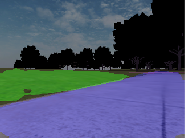
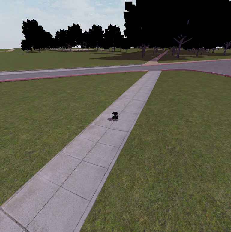
The Baylands simulation and rviz should appear. You should be able to send navigation goals via rviz and the robot should navigate the Baylands world, preferring sidewalks and avoiding grass:

To better see what the plugin is doing, you can enable the segmentation tile map visualization in rviz. This will show a pointcloud of the segmentation observations for each tile, colored by their confidence. Again, you can refer to the picture on the Layer’s README for a visual explanation of how observations are accumulated on the costmap tiles and how that translates to the cost assigned to each tile.

IMPORTANT NOTE: For the sake of simplicity, this tutorial publishes a static transform between the map and odom frames. In a real-world application, you should have a proper localization system (e.g. GPS) to get the map => odom transform.

Conclusion

This tutorial demonstrated how to integrate semantic segmentation with Nav2 for terrain-aware navigation using a pre-trained model that works on Gazebo’s Baylands world and a custom semantic segmentation layer plugin.

To go further, you can train your own model using the Simple Segmentation Toolkit, and tune the costmap parameters to your own application.

Happy terrain-aware navigating!