Mapping and Localization
Now that we have a robot with its sensors set up, we can use the obtained sensor information to build a map of the environment and to localize the robot on the map. The slam_toolbox package is a set of tools and capabilities for 2D Simultaneous Localization and Mapping (SLAM) in potentially massive maps with ROS2. It is also one of the officially supported SLAM libraries in Nav2, and we recommend to use this package in situations you need to use SLAM on your robot setup. Aside from the slam_toolbox, localization can also be implemented through the nav2_amcl package. This package implements Adaptive Monte Carlo Localization (AMCL) which estimates the position and orientation of the robot in a map. Other techniques may also be available, please check Nav2 documentation for more information.
Both the slam_toolbox and nav2_amcl use information from the laser scan sensor to be able to perceive the robot’s environment. Hence, to verify that they can access the laser scan sensor readings, we must make sure that they are subscribed to the correct topic that publishes the sensor_msgs/LaserScan message. This can be configured by setting their scan_topic parameters to the topic that publishes that message. It is a convention to publish the sensor_msgs/LaserScan messages to /scan topic. Thus, by default, the scan_topic parameter is set to /scan. Recall that when we added the lidar sensor to sam_bot in the previous section, we set the topic to which the lidar sensor will publish the sensor_msgs/LaserScan messages as /scan.
In-depth discussions on the complete configuration parameters will not be a scope of our tutorials since they can be pretty complex. Instead, we recommend you to have a look at their official documentation in the links below.
See also
slam_toolbox, see the Github repository of slam_toolbox.nav2_amcl, see the AMCL Configuration Guide.You can also refer to the (SLAM) Navigating While Mapping guide for the tutorial on how to use Nav2 with SLAM. You can verify that slam_toolbox and nav2_amcl have been correctly setup by visualizing the map and the robot’s pose in RViz, similar to what was shown in the previous section.
Costmap 2D
The costmap 2D package makes use of the sensor information to provide a representation of the robot’s environment in the form of an occupancy grid. The cells in the occupancy grid store cost values between 0-254 which denote a cost to travel through these zones. A cost of 0 means the cell is free while a cost of 254 means that the cell is lethally occupied. Values in between these extremes are used by navigation algorithms to steer your robot away from obstacles as a potential field. Costmaps in Nav2 are implemented through the nav2_costmap_2d package.
The costmap implementation consists of multiple layers, each of which has a certain function that contributes to a cell’s overall cost. The package consists of the following layers, but are plugin-based to allow customization and new layers to be used as well: static layer, inflation layer, range layer, obstacle layer, and voxel layer. The static layer represents the map section of the costmap, obtained from the messages published to the /map topic like those produced by SLAM. The obstacle layer includes the objects detected by sensors that publish either or both the LaserScan and PointCloud2 messages. The voxel layer is similar to the obstacle layer such that it can use either or both the LaserScan and PointCloud2 sensor information but handles 3D data instead. The range layer allows for the inclusion of information provided by sonar and infrared sensors. Lastly, the inflation layer represents the added cost values around lethal obstacles such that our robot avoids navigating into obstacles due to the robot’s geometry. In the next subsection of this tutorial, we will have some discussion about the basic configuration of the different layers in nav2_costmap_2d.
The layers are integrated into the costmap through a plugin interface and then inflated using a user-specified inflation radius, if the inflation layer is enabled. For a deeper discussion on costmap concepts, you can have a look at the ROS1 costmap_2D documentation. Note that the nav2_costmap_2d package is mostly a straightforward ROS2 port of the ROS1 navigation stack version with minor changes required for ROS2 support and some new layer plugins.
Build, Run and Verification
We will first launch display.launch.py which launches the robot state publisher that provides the base_link => sensors transformations in our URDF, launches Gazebo that acts as our physics simulator, and provides the odom => base_link from the differential drive plugin or the ekf_node. It also launches RViz which we can use to visualize the robot and sensor information.
Then we will launch slam_toolbox to publish to /map topic and provide the map => odom transform. Recall that the map => odom transform is one of the primary requirements of the Nav2 system. The messages published on the /map topic will then be used by the static layer of the global_costmap.
After we have properly setup our robot description, odometry sensors, and necessary transforms, we will finally launch the Nav2 system itself. For now, we will only be exploring the costmap generation system of Nav2. After launching Nav2, we will visualize the costmaps in RViz to confirm our output.
Launching Description Nodes, RViz and Gazebo
Let us now launch our Robot Description Nodes, RViz and Gazebo through the launch file display.launch.py. Open a new terminal and execute the lines below.
colcon build
. install/setup.bash
ros2 launch sam_bot_description display.launch.py
RViz and the Gazebo should now be launched with sam_bot present in both. Recall that the base_link => sensors transform is now being published by robot_state_publisher and the odom => base_link transform by our Gazebo plugins. Both transforms should now be displayed show without errors in RViz.
Launching slam_toolbox
To be able to launch slam_toolbox, make sure that you have installed the slam_toolbox package by executing the following command:
sudo apt install ros-$ROS_DISTRO-slam-toolbox
We will launch the async_slam_toolbox_node of slam_toolbox using the package’s built-in launch files. Open a new terminal and then execute the following lines:
ros2 launch slam_toolbox online_async_launch.py use_sim_time:=true
The slam_toolbox should now be publishing to the /map topic and providing the map => odom transform.
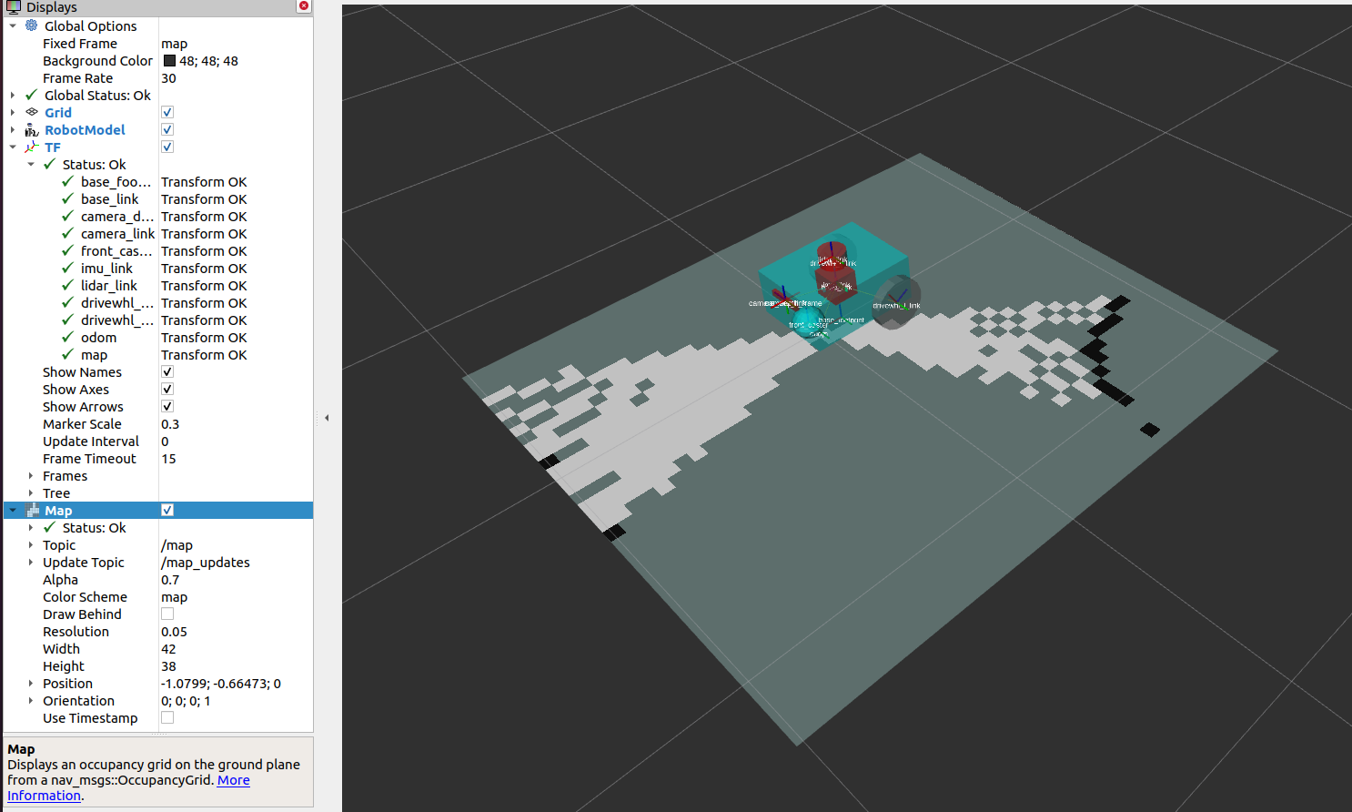
We can verify in RViz that the /map topic is being published. In the RViz window, click the add button at the bottom-left part then go to By topic tab then select the Map under the /map topic. You should be able to visualize the message received in the /map as shown in the image below.
We can also check that the transforms are correct by executing the following lines in a new terminal:
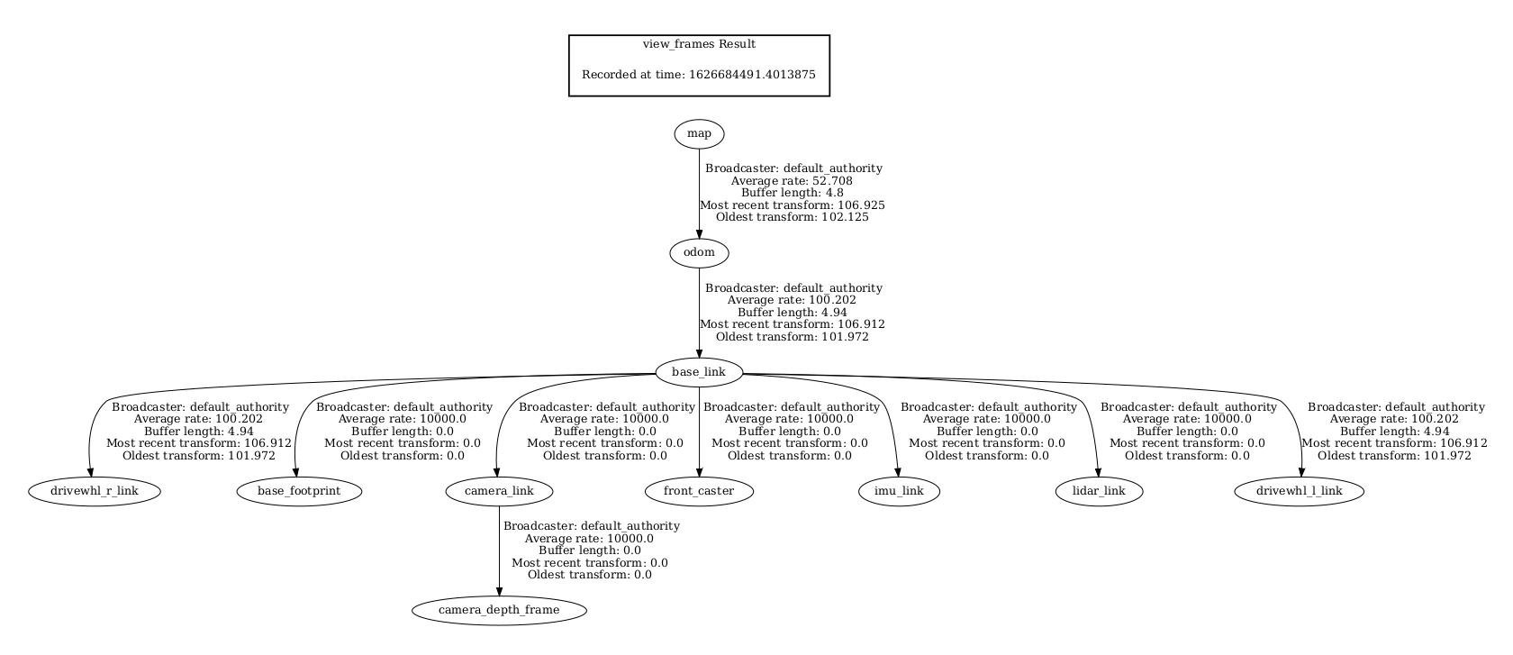
ros2 run tf2_tools view_frames
The line above will create a frames.pdf file that shows the current transform tree. Your transform tree should be similar to the one shown below:
Visualizing Costmaps in RViz
The global_costmap, local_costmap and the voxel representation of the detected obstacles can be visualized in RViz.
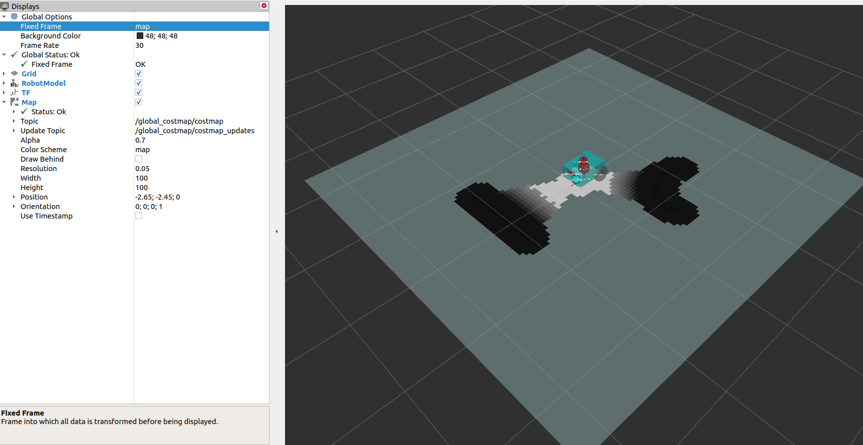
To visualize the global_costmap in RViz, click the add button at the bottom-left part of the RViz window. Go to By topic tab then select the Map under the /global_costmap/costmap topic. The global_costmap should show in the RViz window, as shown below. The global_costmap shows areas which should be avoided (black) by our robot when it navigates our simulated world in Gazebo.
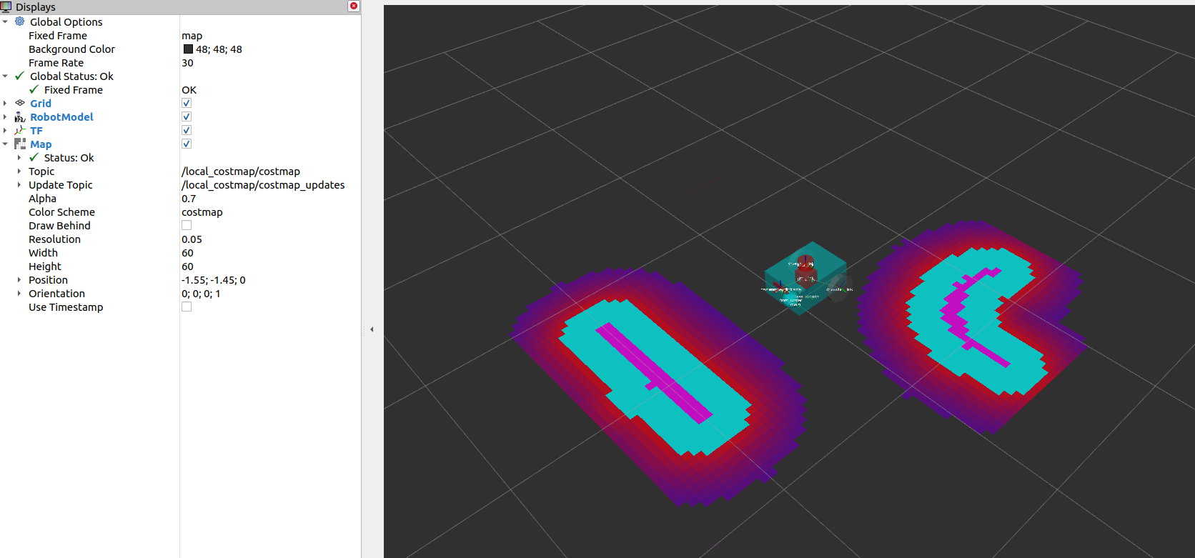
To visualize the local_costmap in RViz, select the Map under the /local_costmap/costmap topic. Set the color scheme in RViz to costmap to make it appear similar to the image below.
To visualize the voxel representation of the detected object, open a new terminal and execute the following lines:
ros2 run nav2_costmap_2d nav2_costmap_2d_markers voxel_grid:=/local_costmap/voxel_grid visualization_marker:=/my_marker
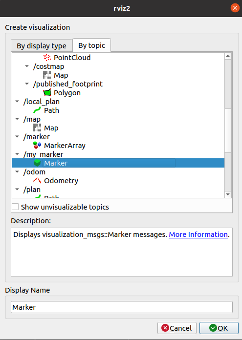
The line above sets the topic where the the markers will be published to /my_marker. To see the markers in RViz, select Marker under the /my_marker topic, as shown below.
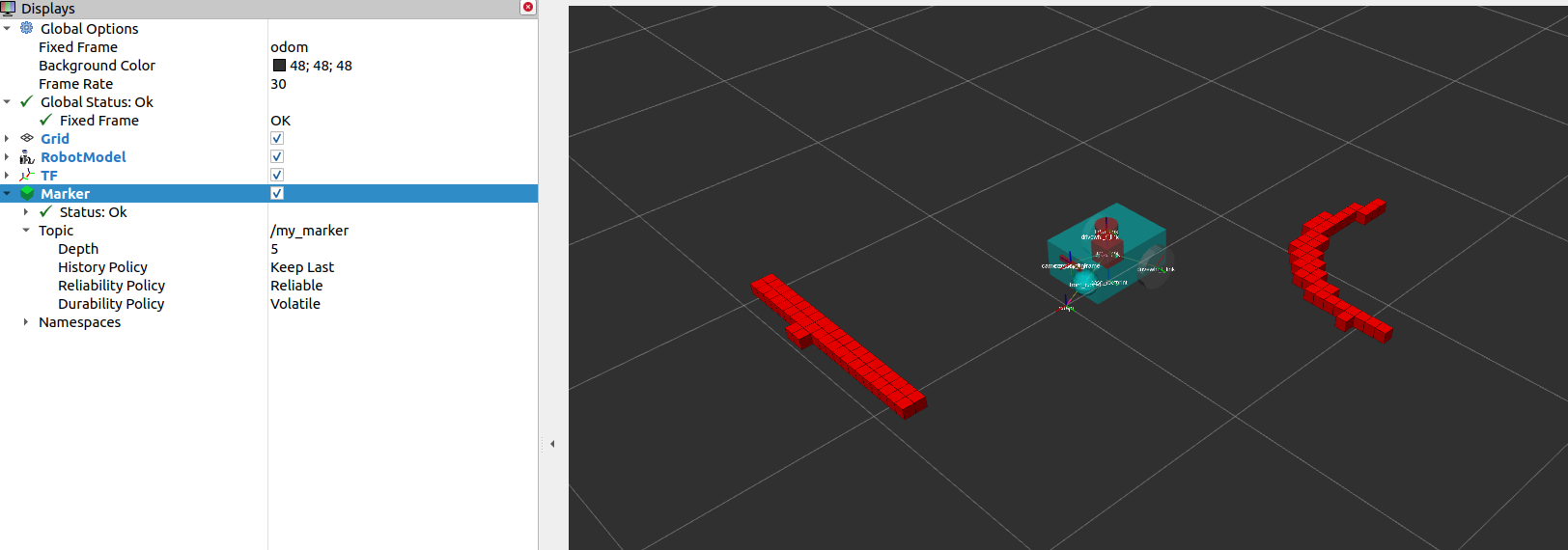
Then set the fixed frame in RViz to odom and you should now see the voxels in RViz, which represent the cube and the sphere that we have in the Gazebo world:
Conclusion
In this section of our robot setup guide, we have discussed the importance of sensor information for different tasks associated with Nav2. More specifically, tasks such as mapping (SLAM), localization (AMCL), and perception (costmap) tasks.
Then, we set up a basic configuration for the nav2_costmap_2d package using different layers to produce a global and local costmap. We then verify our work by visualizing these costmaps in RViz.